I_x about the X axis and I_y about the Y axis, valid for any view: plan, transverse section or profile*

1. Convention: set this up first

Draw the view you are looking at. Then fix the axes as follows. The formulas depend only on this convention, so they hold for every view.

• X axis: the line along which the stations are equally spaced (interval h) and from which every ordinate is measured.
• Y axis: the line perpendicular to X at station 0. Levers are measured from it.
• y: ordinate (offset) from the X axis to the edge of the shape at each station.
• n: lever, the station number counted from the Y axis, so x = n·h.
• SM: Simpson multiplier.
• k: number of sides of the X axis on which the shape lies (k = 1 for one side only; k = 2 for a shape symmetrical about X when half ordinates are given).
• To look at the shape from another direction, rotate the drawing until the stations run along X, then reuse the same formulas.

---

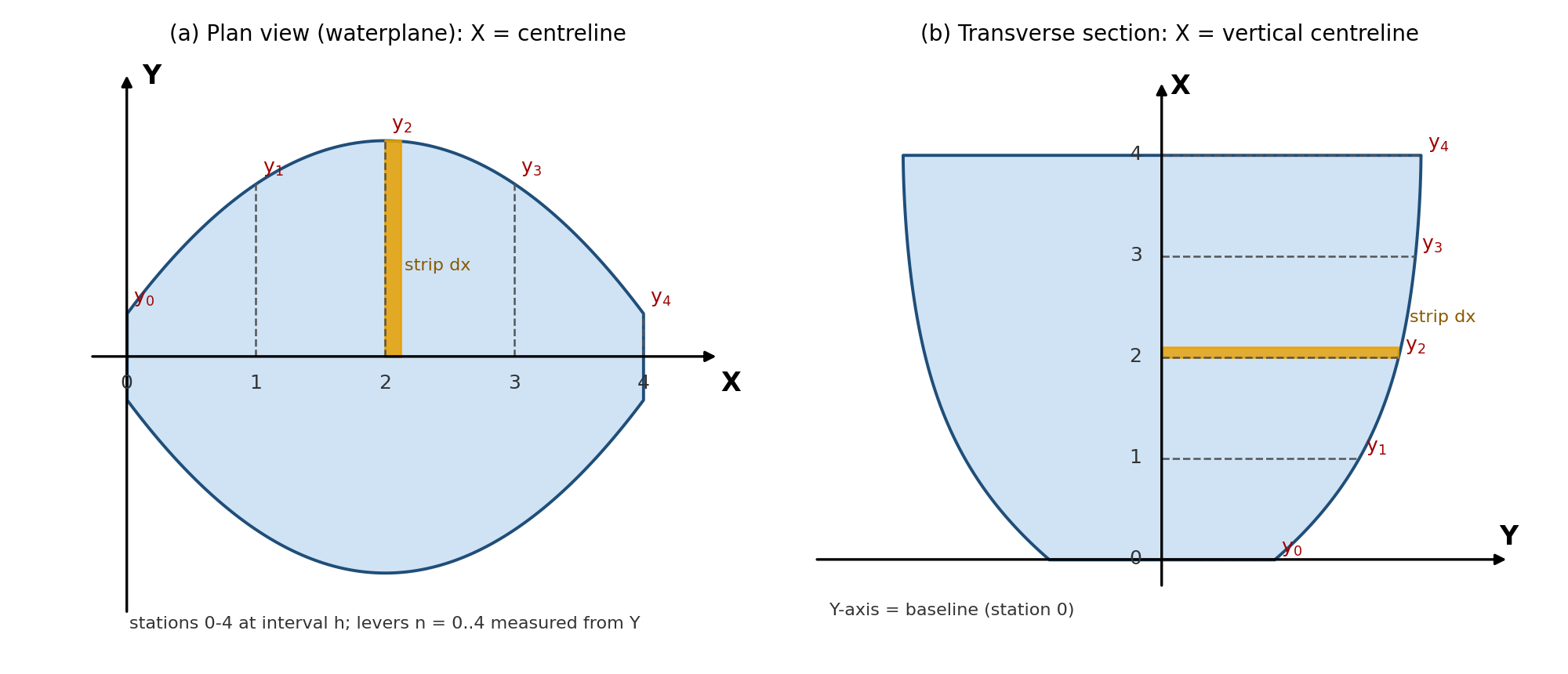
2. Basic integrals (per strip of width dx)

About X Axis

Strip area $dA = y \times dx$. Its own inertia about its base is $dI_x = \frac{y^3}{12} \times dx$, and moving it by $\frac {y}{2}$ (parallel axis theorem) adds $y \times dx \times \frac {y^2}{2^2}$. Together:

$$dI_x = (\frac {y^3}{12}+ \frac {y^3}{4})\times dx$$

About Y Axis

About the Y axis the strip sits at distance x, so $dI_y = x^2 \times y \times dx$. The strip’s own term $y\times \frac {dx^3}{12}$ is negligible as dx → 0 and is dropped. Hence, for k sides:

$$A = k \int y dx$$

$$I_x = \frac{k}{3} \int y^3 dx$$

$$I_y = {k} \int x^2 y dx$$

---

3. Simpson’s form

Let $c = \frac {h}{3}$ for Simpson’s 1st rule (SM = 1, 4, 2, 4, … 4, 1; needs an odd number of ordinates) or $c = \frac {3h}{8}$ for the 2nd rule (SM = 1, 3, 3, 2, 3, 3, … 3, 1; needs the number of intervals to be a multiple of 3). With levers in whole intervals (x = n·h):

Quantity	Working formula
Area	A = k·c·Σ(SM·y) $A = k \times c \times \Sigma (SM \times y)$
Ix: about the X axis	Ix = (k·c/3)·Σ(SM·y³) $I_x = ( k \times \frac {c}{3}) \times \Sigma (SM \times y^3)$
Iy: about the Y axis (station 0)	Iy = k·c·h²·Σ(SM·y·n²) $I_y = k \times c \times h^2 \times \Sigma ( SM \times y \times n^2)$
Centroid distance from Y axis	x̄ = h·Σ(SM·y·n) / Σ(SM·y) $\bar x = h \times \frac {\Sigma (SM \times y \times n)}{ \Sigma (SM \times y)}$
Iy about the centroid	Iy,cg = Iy − A·x̄² $I_{yCG} = I_y - (A \times \bar x ^2)$
Ix about the centroid (k = 1)	Ix,cg = Ix − A·ȳ², with ȳ = ½·Σ(SM·y²) / Σ(SM·y) $I_{xCG}= I_x - (A\times \bar y ^2)$ with $\bar y = \frac {1}{2} \times \frac{\Sigma (SM \times y^2)}{\Sigma (SM \times y)}$
Ix about the centroid (k = 2, symmetrical about X)	ȳ = 0, so Ix is already the centroidal value

For Simpson’s 1st rule these reduce to:

Ix = (k·h/9)·Σ(SM·y³)

$$I_x = (k \times \frac{h}{9}) \times \Sigma (SM \times y^3)$$

Iy = (k·h³/3)·Σ(SM·y·n²)

$$I_y = (k \times \frac {h^3}{9})\times \Sigma ( SM \times \times n ^2)$$

The levers n already include h, which is why the extra $h^2$ ( $h^3$overall) appears.

---

4. Mapping to the view you are looking at

View	X axis, stations, y	k	Ix means	Iy means
Plan view (waterplane)	X = centreline, stations from aft to forward, y = half-breadth	2	Transverse $I_T$ about the centreline. $BM_T = \frac {I_T}{\nabla}$	About the transverse axis at station 0. Shift to the CoF: $I_L = I_y − A·x_F^2$. $BM_L = \frac {I_L}{\nabla}$
Transverse section (looking fore/aft)	X = vertical centreline, stations = waterlines from the baseline, y = half-breadth	2	Section area about the vertical centreline	Section area about the baseline. Shift to the area centroid with x̄
Profile (side view)	X = keel line, stations along the length, y = depth	1	Area about the keel line (shift with ȳ)	Area about the vertical axis at station 0 (shift with x̄)

Rule of thumb: $I_x$ always uses the cube of the ordinate $y^3$. $I_y$ always uses the ordinate times the square of the lever $y \times n^2$.

---

5. Worked example (plan view, Y axis at the after end)

Waterplane with 5 stations, h = 5 m, half-breadths y = 1, 4, 5, 4, 1 m, k = 2, Simpson’s 1st rule.

Stn	n	y	SM	SM·y	SM·y·n	SM·y·n²	y³	SM·y³
0	0	1	1	1	0	0	1	1
1	1	4	4	16	16	16	64	256
2	2	5	2	10	20	40	125	250
3	3	4	4	16	48	144	64	256
4	4	1	1	1	4	16	1	1
Σ				44	88	216		764

• A = 2·(5/3)·44 = 146.67 m²
• Ix = (2·5/9)·764 = 848.89 m⁴ (centreline, already centroidal because the shape is symmetrical)
• x̄ = 5·88/44 = 10.0 m from the Y axis
• Iy about station 0 = 2·(5³/3)·216 = 18 000 m⁴
• Iy,cg = 18 000 − 146.67·10.0² = 3 333.33 m⁴

Self-check on a rectangle of length 4h and full breadth 2y (Σ SM·y³ = 12y³): the formula gives Ix = (2h/9)·12y³ = 8hy³/3, which equals the exact (1/12)(2y)³(4h). About the end, Σ(SM·n²) = 64 gives Iy = 128·y·h³/3, also exact. Simpson’s rules are exact here because the integrands are polynomials of degree 3 or lower.

---

6. Common errors

• Cubing after applying the multiplier: use SM·y³, not (SM·y)³.
• Forgetting k when half ordinates are used.
• Using y² in the Iy column. It is the ordinate to the first power times the lever squared.
• Dropping the h² (or h³) when the levers are written as station numbers.
• Quoting Iy about an arbitrary axis as if it were about the centroid or the centre of flotation. Always apply −A·x̄² (or −A·x_F²).
• Using Simpson’s 1st rule with an even number of ordinates.